rating-gp (prototype)#

rating-gp is a prototype model that can fit rating curves (stage-discharge relationship) using a Gaussian process. This model seeks to expand the typical rating curve fitting process to include shifts in the rating curve with time such that the time evolution in the rating curve can be included in the model.

%load_ext autoreload
%autoreload 2

#!pip install discontinuum[rating_gp]

import matplotlib.pyplot as plt
import numpy as np
import xarray as xr
import pandas as pd

%matplotlib inline

USGS site 10154200#

Let’s select a site that has a nice variation in the rating curve with time. For this example, we will use USGS site 10154200, as it has a very clear shifting with time.

site = '10154200'

# Select a date range
start_date = "1988-10-01" 
end_date = "2021-09-30"

Now that we have selected our site, we need to download the data. In discontinuum, the convention is to download directly using providers, which wrap a data provider’s web-service and perform some initial formatting and metadata construction, then return the result as an xarray.Dataset. Here, we use the usgs provider. If you need data from another source, create a provider and ensure the output matches that of the usgs provider. Here, we’ll download some instantaneous stage data to use as our model’s input, and some discharge data as our target.

With the training data, we’re now ready to fit a model to the site. Depending on your hardware, this should take about 10s.

%%time
# select an engine
from rating_gp.models.gpytorch import RatingGPMarginalGPyTorch as RatingGP

model = RatingGP()
model.fit(target=training_data['discharge'],
          covariates=training_data[['stage']],
          target_unc=training_data['discharge_unc'],
          iterations=2000,
          early_stopping=True,
          )

/opt/hostedtoolcache/Python/3.13.5/x64/lib/python3.13/site-packages/sklearn/pipeline.py:61: FutureWarning: This Pipeline instance is not fitted yet. Call 'fit' with appropriate arguments before using other methods such as transform, predict, etc. This will raise an error in 1.8 instead of the current warning.
  warnings.warn(

/opt/hostedtoolcache/Python/3.13.5/x64/lib/python3.13/site-packages/linear_operator/utils/cholesky.py:40: NumericalWarning: A not p.d., added jitter of 1.0e-06 to the diagonal
  warnings.warn(
/opt/hostedtoolcache/Python/3.13.5/x64/lib/python3.13/site-packages/linear_operator/utils/cholesky.py:40: NumericalWarning: A not p.d., added jitter of 1.0e-05 to the diagonal
  warnings.warn(
/opt/hostedtoolcache/Python/3.13.5/x64/lib/python3.13/site-packages/linear_operator/utils/cholesky.py:40: NumericalWarning: A not p.d., added jitter of 1.0e-04 to the diagonal
  warnings.warn(
/opt/hostedtoolcache/Python/3.13.5/x64/lib/python3.13/site-packages/linear_operator/operators/_linear_operator.py:2163: NumericalWarning: Runtime Error when computing Cholesky decomposition: Matrix not positive definite after repeatedly adding jitter up to 1.0e-04.. Using symeig method.
  warnings.warn(

Early stopping triggered after 437 iterations
Best objective: -1.085162
CPU times: user 35.2 s, sys: 284 ms, total: 35.4 s
Wall time: 18.4 s

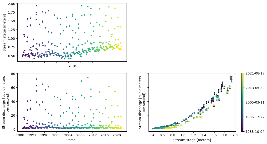
With the model fit, we can generate some nice plots of an observed rating curve and time series of both stage and discharge.

fig, ax = plt.subplots(2, 2, figsize=(13, 7), sharex='col', sharey='row')
ax[0, 0] = model.plot_stage(ax=ax[0, 0])
ax[1, 0] = model.plot_discharge(ax=ax[1, 0])
ax[1, 1] = model.plot_observed_rating(ax=ax[1, 1], zorder=3)
_ = ax[0, 1].axis('off')
_ = model.add_time_colorbar(ax=ax[1, 1])

../_images/8e51dbe4183e379d820a51dd441b06c27fa62bd2a7b413b8c953c733d702cf52.png

One major advantage of rating-gp is that the resulting model can be used to make predictions of a rating curve at any moment in time. To see how well our model can predict a rating curve across time, let’s plot the rating curves at an interval of every 5 years at the start of a water year (i.e., October 1st). This way we can see how well the model accounts for any shift in the rating with time.

import warnings
warnings.filterwarnings('ignore')

fig, ax = plt.subplots(1, 1, figsize=(7.5, 5))
ax = model.plot_ratings_in_time(ax=ax, time=pd.date_range('1990', '2021', freq='5YS-OCT'))
ax = model.plot_ratings_in_time(ax=ax, time=['2020-10-01'], ci=0.95)
ax = model.plot_observed_rating(ax, zorder=3)
ax.set_xscale('log')
ax.set_yscale('log')

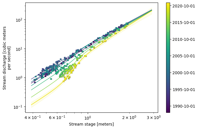
../_images/e2f734a0a92f9e785285987a6e9c3a8b8fd5ca48a693a86116811f12d7b2edac.png

Nice! The shifts with time are clearly predicted by the model. These results are are promising for rating-gp to be able to model shift in rating curves effectively.

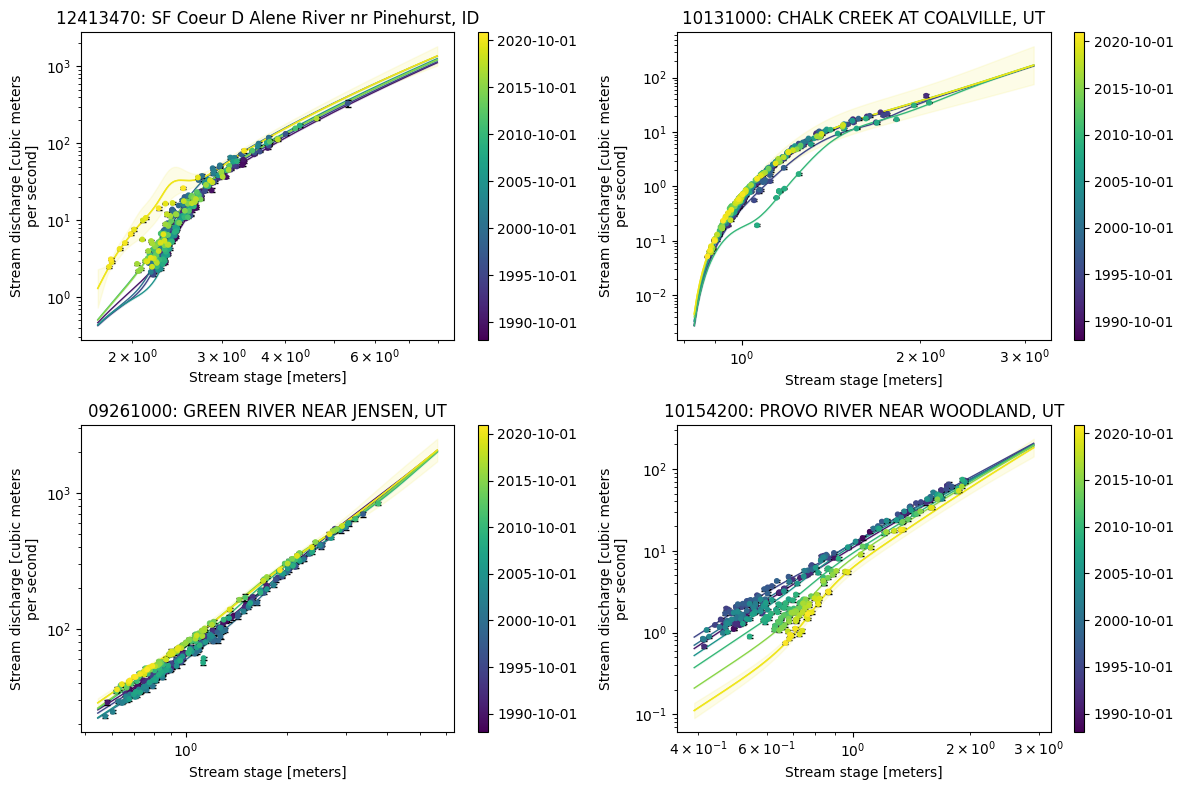
Multi-site Example#

As a final show of how well rating-gp works, let’s select some sites that have a nice variety of rating curves, rather then a single one. We will include ones with clear breaks and shifts and others without breaks and minimal shifts. USGS site number 12413470 is a good example of a rating with a clear break around a stage of 2.7m and very recent and drastic shift. 10131000 is another good example of a rating with a break, but no real shifts in time. 09261000 is a site with no breaks and minimal shifts making it an ideal basic example. Finally, we will keep 10154200 as it has no prominent breaks, but it does have a very clear shifting with time. Therefore, these four sites should be a nice standard for testing how rating-gp performs on different rating curves.

sites = {"12413470": 'SF Coeur D Alene River nr Pinehurst, ID',
         '10131000': 'CHALK CREEK AT COALVILLE, UT',
         '09261000': 'GREEN RIVER NEAR JENSEN, UT',
         '10154200': 'PROVO RIVER NEAR WOODLAND, UT'}

Now that we have our sites, we need to download the data using the USGS provider.

training_data_dict = {}
for site in sites:
    training_data_dict[site] = usgs.get_measurements(site=site, start_date=start_date, end_date=end_date)

With the training data, we’re now ready to fit a model to each site. Depending on your hardware, this should take about 10-20s for each site.

%%time
model = {}
for site in sites:
    training_data = training_data_dict[site]
    model[site] = RatingGP()
    model[site].fit(target=training_data['discharge'],
                    covariates=training_data[['stage']],
                    target_unc=training_data['discharge_unc'],
                    iterations=2000,
                    early_stopping=True,
                    )

Early stopping triggered after 928 iterations
Best objective: -0.555369

Early stopping triggered after 1359 iterations
Best objective: -1.011360

Early stopping triggered after 469 iterations
Best objective: -1.436839

Early stopping triggered after 433 iterations
Best objective: -1.094050
CPU times: user 4min 3s, sys: 942 ms, total: 4min 4s
Wall time: 2min 2s

Now that we have our models fit, let’s plot all of the rating curves in time as we did above. We will again predict each rating at an interval of every 5 years at the start of a water year (i.e., October 1st) in 1990.

fig, axes = plt.subplots(2, 2, figsize=(12, 8))
for site, ax in zip(sites, axes.flatten()):
    ax = model[site].plot_ratings_in_time(ax=ax, time=pd.date_range('1990', '2021', freq='5YS-OCT'))    
    ax = model[site].plot_ratings_in_time(ax=ax, time=['2020-10-01'], ci=0.95)    
    ax = model[site].plot_observed_rating(ax, zorder=3)
    ax.set_xscale('log')
    ax.set_yscale('log')
    ax.set_title(f'{site}: {sites[site]}')

plt.tight_layout()

rating-gp (prototype)

Contents

rating-gp (prototype)#

USGS site 10154200#

Multi-site Example#