loadest-gp (prototype)

LOAD ESTimator (LOADEST) is a software program for estimating some constituent using surrogate variables (covariates). However, LOADEST has several serious limitations, and it has been all but replaced by another model known as Weighted Regressions on Time, Discharge, and Season (WRTDS). loadest-gp essentially reimplements WRTDS as a Gaussian process.

# install the latest version of discontinuum
# !pip install discontinuum[loadest_gp]
%load_ext autoreload
%autoreload 2

import matplotlib.pyplot as plt
import xarray as xr

%matplotlib inline

# setup

# SF Coeur D Alene River 
#site = "12413470"
#start_date = "1988-10-01" 
#end_date = "2021-09-30" 

# Choptank River at Greensboro, MD
site = "01491000" 
start_date = "1979-10-01"
end_date = "2011-09-30"

characteristic = 'Inorganic nitrogen (nitrate and nitrite)'
fraction = 'Dissolved'

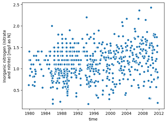
First, download the data. In discontinuum, the convention is to download directly using providers, which wrap a data provider’s web-service and perform some initial formatting and metadata construction, then return the result as an xarray.Dataset. Here, we use the usgs provider. If you need data from another source, create a provider and ensure the output matches that of the usgs provider. We’ll download some daily streamflow data to use as our model’s input, and some concentration samples as our target.

from loadest_gp.providers import usgs

# download covariates (daily streamflow)
daily = usgs.get_daily(site=site, start_date=start_date, end_date=end_date)

# download target (concentration)
samples = usgs.get_samples(site=site, 
                           start_date=start_date, 
                           end_date=end_date, 
                           characteristic=characteristic, 
                           fraction=fraction)

samples

/home/runner/work/discontinuum/discontinuum/src/loadest_gp/providers/usgs.py:255: UserWarning: Censored values have been removed from the dataset.
  warnings.warn(

<xarray.Dataset> Size: 10kB
Dimensions:        (time: 652)
Coordinates:
  * time           (time) datetime64[ns] 5kB 1979-12-05T10:30:00 ... 2011-04-...
Data variables:
    concentration  (time) float64 5kB 1.4 0.62 1.2 1.2 ... 0.92 1.54 1.39 0.99
Attributes:
    id:         01491000
    name:       CHOPTANK RIVER NEAR GREENSBORO, MD
    latitude:   38.99719444
    longitude:  -75.7858056

xarray.Dataset

• Dimensions:
  • time: 652
• Coordinates: (1)
  • time
    (time)
    datetime64[ns]
    1979-12-05T10:30:00 ... 2011-04-...

    array(['1979-12-05T10:30:00.000000000', '1979-10-24T10:30:00.000000000',
           '1979-12-21T11:30:00.000000000', ..., '2011-08-09T10:00:00.000000000',
           '2011-07-13T09:30:00.000000000', '2011-04-13T11:00:00.000000000'],
          shape=(652,), dtype='datetime64[ns]')

• Data variables: (1)
  • concentration
    (time)
    float64
    1.4 0.62 1.2 1.2 ... 1.54 1.39 0.99

    pcode :

    00631

    standard_name :

    concentration

    long_name :

    Inorganic nitrogen (nitrate and nitrite)

    units :

    mg/l as N

    suffix :

    conversion :

    1.0

    array([1.4  , 0.62 , 1.2  , 1.2  , 1.1  , 0.93 , 0.62 , 1.1  , 1.   ,
           0.84 , 1.1  , 1.   , 1.   , 0.81 , 0.69 , 0.98 , 1.3  , 1.2  ,
           0.94 , 0.6  , 0.88 , 0.82 , 1.3  , 1.1  , 1.4  , 0.99 , 1.4  ,
           1.2  , 1.1  , 1.2  , 1.4  , 0.56 , 1.2  , 0.83 , 1.1  , 1.   ,
           1.3  , 1.2  , 1.1  , 1.4  , 0.72 , 0.57 , 0.29 , 0.56 , 0.83 ,
           0.77 , 0.83 , 0.7  , 0.92 , 2.   , 0.67 , 0.78 , 0.88 , 1.4  ,
           1.5  , 0.28 , 0.94 , 1.3  , 0.18 , 0.91 , 1.5  , 1.   , 1.2  ,
           1.1  , 1.   , 1.5  , 1.2  , 0.88 , 0.77 , 1.   , 0.92 , 1.1  ,
           0.54 , 0.71 , 1.4  , 1.   , 1.2  , 0.67 , 0.95 , 1.3  , 1.   ,
           0.93 , 1.4  , 1.   , 1.2  , 1.1  , 1.1  , 0.94 , 0.97 , 0.98 ,
           1.1  , 1.1  , 0.93 , 1.4  , 1.5  , 1.3  , 0.99 , 0.97 , 0.84 ,
           0.8  , 0.79 , 0.77 , 1.1  , 1.1  , 0.97 , 0.67 , 1.6  , 1.1  ,
           1.   , 0.9  , 0.86 , 1.2  , 0.95 , 1.3  , 0.23 , 1.1  , 0.78 ,
           1.8  , 1.2  , 0.9  , 0.84 , 0.85 , 0.58 , 1.1  , 1.4  , 0.58 ,
           0.56 , 1.4  , 1.7  , 1.3  , 0.9  , 1.3  , 0.89 , 1.5  , 0.84 ,
           1.6  , 0.71 , 1.2  , 0.8  , 1.7  , 1.4  , 1.   , 1.   , 0.7  ,
           1.2  , 1.8  , 1.1  , 0.93 , 1.5  , 1.1  , 1.3  , 0.98 , 1.1  ,
           1.2  , 0.84 , 1.2  , 0.8  , 1.2  , 0.65 , 0.94 , 0.84 , 1.1  ,
           0.91 , 0.82 , 1.1  , 0.52 , 0.94 , 1.   , 1.2  , 0.86 , 0.96 ,
           0.97 , 0.68 , 1.6  , 0.4  , 1.4  , 0.88 , 1.   , 1.2  , 1.4  ,
    ...
           0.64 , 1.23 , 1.51 , 1.81 , 1.28 , 0.97 , 0.73 , 0.96 , 0.9  ,
           1.06 , 0.65 , 2.09 , 1.53 , 1.47 , 1.17 , 1.76 , 1.48 , 1.38 ,
           1.13 , 1.24 , 0.97 , 1.27 , 1.01 , 1.23 , 0.39 , 2.   , 1.76 ,
           0.85 , 1.6  , 0.97 , 1.44 , 1.27 , 1.41 , 0.76 , 1.05 , 0.87 ,
           0.43 , 1.42 , 1.28 , 1.51 , 1.18 , 1.27 , 0.75 , 1.42 , 0.98 ,
           0.94 , 1.18 , 1.1  , 1.67 , 1.28 , 2.17 , 1.54 , 0.86 , 1.15 ,
           1.13 , 1.43 , 1.72 , 0.6  , 1.54 , 1.38 , 1.32 , 1.18 , 1.23 ,
           1.63 , 1.38 , 1.46 , 1.49 , 1.37 , 0.74 , 1.04 , 1.7  , 1.26 ,
           1.14 , 1.34 , 0.98 , 1.93 , 1.15 , 0.97 , 1.75 , 1.75 , 1.87 ,
           1.18 , 1.33 , 1.17 , 1.29 , 2.17 , 1.51 , 0.62 , 1.46 , 1.14 ,
           1.68 , 1.1  , 1.35 , 1.42 , 1.66 , 1.66 , 1.29 , 2.36 , 0.56 ,
           1.37 , 1.59 , 0.87 , 1.52 , 1.06 , 1.58 , 1.74 , 1.59 , 1.27 ,
           1.12 , 1.46 , 0.6  , 1.56 , 1.29 , 0.93 , 1.62 , 0.7  , 1.25 ,
           2.14 , 1.4  , 1.64 , 1.43 , 1.59 , 1.36 , 1.69 , 0.31 , 0.3  ,
           1.54 , 0.31 , 1.59 , 0.97 , 1.29 , 0.95 , 1.49 , 1.04 , 1.22 ,
           1.08 , 0.57 , 1.86 , 1.55 , 1.18 , 0.72 , 1.66 , 0.74 , 2.43 ,
           1.74 , 1.78 , 0.75 , 1.43 , 1.46 , 1.21 , 1.54 , 0.69 , 1.6  ,
           1.26 , 1.51 , 1.13 , 0.85 , 1.81 , 1.36 , 1.02 , 1.44 , 1.18 ,
           1.8  , 0.78 , 1.23 , 0.94 , 0.57 , 1.74 , 0.2  , 0.97 , 0.8  ,
           0.92 , 1.54 , 1.39 , 0.99 ])

• Indexes: (1)
  • time
    PandasIndex

    PandasIndex(DatetimeIndex(['1979-12-05 10:30:00', '1979-10-24 10:30:00',
                   '1979-12-21 11:30:00', '1980-02-25 11:45:00',
                   '1980-09-08 10:30:00', '1980-07-28 10:40:00',
                   '1980-10-29 10:45:00', '1980-06-24 10:45:00',
                   '1980-05-27 10:50:00', '1980-01-24 10:30:00',
                   ...
                   '2011-02-03 09:45:00', '2011-04-18 09:00:00',
                   '2011-06-14 10:30:00', '2011-08-30 10:00:00',
                   '2011-03-07 11:45:00', '2011-09-29 08:30:00',
                   '2011-08-15 10:25:00', '2011-08-09 10:00:00',
                   '2011-07-13 09:30:00', '2011-04-13 11:00:00'],
                  dtype='datetime64[ns]', name='time', length=652, freq=None))

• Attributes: (4)

  id :

  01491000

  name :

  CHOPTANK RIVER NEAR GREENSBORO, MD

  latitude :

  38.99719444

  longitude :

  -75.7858056

_ = samples.plot.scatter(x='time', y='concentration')

Next, prepare the training data by performing an inner join of the target and covariates.

from discontinuum.utils import aggregate_to_daily

samples = aggregate_to_daily(samples)

training_data = xr.merge([samples, daily], join='inner')

Now, we’re ready to fit the model. Depending on your hardware, this can take seconds to several minutes. The first fit will also compile the model, which takes longer. After running it once, try running the cell again and note the difference in wall time.

%%time
# select an engine
# from loadest_gp import LoadestGPMarginalPyMC as LoadestGP
from loadest_gp import LoadestGPMarginalGPyTorch as LoadestGP

model = LoadestGP()

model.fit(target=training_data['concentration'], covariates=training_data[['time','flow']])

CPU times: user 7.01 s, sys: 610 ms, total: 7.62 s
Wall time: 4.35 s

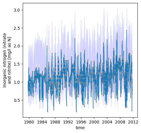
# plot result
_ = model.plot(daily[['time','flow']])

/opt/hostedtoolcache/Python/3.13.5/x64/lib/python3.13/site-packages/gpytorch/likelihoods/gaussian_likelihood.py:347: GPInputWarning: You have passed data through a FixedNoiseGaussianLikelihood that did not match the size of the fixed noise, *and* you did not specify noise. This is treated as a no-op.
  warnings.warn(
/opt/hostedtoolcache/Python/3.13.5/x64/lib/python3.13/site-packages/sklearn/pipeline.py:61: FutureWarning: This Pipeline instance is not fitted yet. Call 'fit' with appropriate arguments before using other methods such as transform, predict, etc. This will raise an error in 1.8 instead of the current warning.
  warnings.warn(

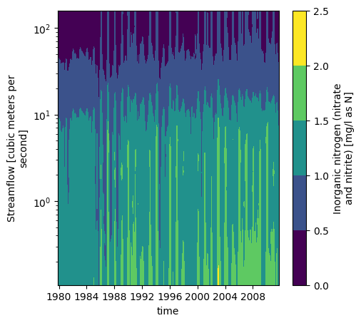
Like WRTDS, we can also plot the variable space:

_ = model.contourf(levels=5, y_scale='log')

/opt/hostedtoolcache/Python/3.13.5/x64/lib/python3.13/site-packages/gpytorch/likelihoods/gaussian_likelihood.py:347: GPInputWarning: You have passed data through a FixedNoiseGaussianLikelihood that did not match the size of the fixed noise, *and* you did not specify noise. This is treated as a no-op.
  warnings.warn(

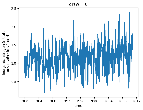
For plotting, we don’t need to simulate the full covariance matrix. Instead, we can use its diagonal to compute confidence intervals, but for most other uses, we need to simulate predictions using full covariance, which is slower. Here, we simulate daily concentration during 1980-2010, then we will use those simulations to estimate annual fluxes with uncertainty.

# simulate concentration
sim_slice = daily[['time','flow']].sel(time=slice("1980","2010"))

sim = model.sample(sim_slice)

# plot the first realization of concentration. 
_ = sim.sel(draw=0).plot.line(x='time')

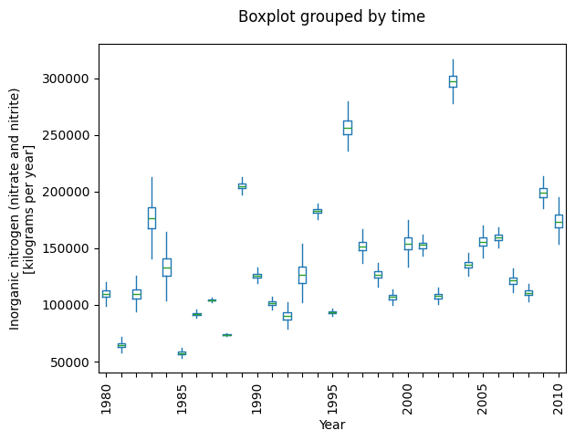
In practice, we aren’t interested in a single simulated timeseries. Rather, we take a large sample of simulated series, then pass them through some function to simulate a probability distribution. For example, if we were interested in some annual value we would pass the simulations through that annual function to estimate a probability distribution. We demonstrate this concept for estimating the annual nutrient flux.

loadest_gp provides a couple of convenience functions just for this purpose.

from loadest_gp.utils import concentration_to_flux, plot_annual_flux

flux = concentration_to_flux(sim, sim_slice['flow'])
_ = plot_annual_flux(flux)

In most streams, flow varies substantially from year-to-year, and we’d like to know what the flux might have been had flow been constant. In causal parlance, this is refered to as a counterfactual. However,loadest_gp isn’t a causal model and can’t provide us with counterfactuals. In other words, it can interpolate but not extrapolate. Nevertheless, we may treat it as a causal model and see what happens. Think of this type of analysis as a pseudo-counterfactual or educated guessing. There are a variety of strategies that we might employee, some more sophisticated then others. At the end of the day, remember we’re only guessing, so keep it simple and don’t be tempted into over-interpretation. Here, we’ll use a simple time substitution. Pick one year’s worth of data and repeat it (except for the time variable) over the entire period of analysis. For example, let’s repeat the year 1995 to fill in the data for our 1980-2010 in our counterfactual. What’s special about 1995? Nothing, except that it is at the middle of our period. Choosing a different year should give similar results.

# create the pseudo-counterfactual
from discontinuum.utils import time_substitution

counterfactual = time_substitution(sim_slice, interval=slice("1995","1995"))

# simulate
counterfactual_sim = model.sample(counterfactual)
counterfactual_flux = concentration_to_flux(counterfactual_sim, sim_slice['flow'])

# and plot the result
_ = plot_annual_flux(counterfactual_sim)

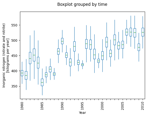
Now, the annual fluxes should be less variable than before, and the trend becomes apparent (depending on your choice of river).