Natural Splines#
Splines are flexible functions that can be used to fit rating curves. In fact, the multi-segment power law is a form of linear spline, but other types of spline can be used as well. One alternative is the natural spline. They have the advantage of being faster to fit, but their form is less constrained than the segmented power law. As a result, natural splines may produce strange results, particularly with small datasets.
%load_ext autoreload
%autoreload 2

import pymc as pm
import arviz as az
from ratingcurve.ratings import PowerLawRating, SplineRating

import numpy as np

from ratingcurve import data
data.list()
WARNING (pytensor.tensor.blas): Using NumPy C-API based implementation for BLAS functions.
['chalk artificial',
 'co channel',
 'green channel',
 'provo natural',
 '3-segment simulated',
 'mahurangi artificial',
 'nordura',
 'skajalfandafljot',
 'isere']
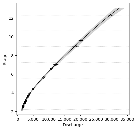
Green River#
In practice splines can work quite well, particularly for simpler ratings. Here is an example showing a natural spline fit to the Green River dataset.
df = data.load('green channel')

spline = SplineRating(df=8)
# converges much faster than the power law
trace = spline.fit(q=df['q'],
                   h=df['stage'],
                   q_sigma=df['q_sigma'],
                   n=70_000)

spline.plot()
/opt/hostedtoolcache/Python/3.11.9/x64/lib/python3.11/site-packages/rich/live.py:231: UserWarning: install
"ipywidgets" for Jupyter support
  warnings.warn('install "ipywidgets" for Jupyter support')
Finished [100%]: Average Loss = -39.368
Sampling: [model_q, sigma, w]
Sampling: [model_q]
/opt/hostedtoolcache/Python/3.11.9/x64/lib/python3.11/site-packages/rich/live.py:231: UserWarning: install
"ipywidgets" for Jupyter support
  warnings.warn('install "ipywidgets" for Jupyter support')
Sampling: [model_q]
/opt/hostedtoolcache/Python/3.11.9/x64/lib/python3.11/site-packages/rich/live.py:231: UserWarning: install
"ipywidgets" for Jupyter support
  warnings.warn('install "ipywidgets" for Jupyter support')
Simulated Rating#
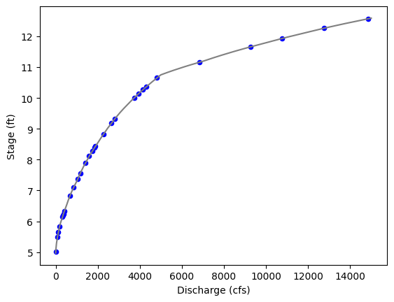
sim_df = data.load('3-segment simulated')

# subsample the simulated rating curve
n_sample = 30
df = sim_df.sample(n_sample, random_state=12345)

ax = sim_df.plot(x='q', y='stage', color='gray', ls='-', legend=False)
df.plot.scatter(x='q', y='stage', marker='o', color='blue', ax=ax)
ax.set_xlabel("Discharge (cfs)")
ax.set_ylabel("Stage (ft)")
Text(0, 0.5, 'Stage (ft)')
spline = SplineRating(df=10)
trace = spline.fit(q=df['q'],
                   h=df['stage'],
                   n=100_000)

spline.plot()
/opt/hostedtoolcache/Python/3.11.9/x64/lib/python3.11/site-packages/rich/live.py:231: UserWarning: install
"ipywidgets" for Jupyter support
  warnings.warn('install "ipywidgets" for Jupyter support')
Finished [100%]: Average Loss = -2.8101
Sampling: [model_q, sigma, w]
Sampling: [model_q]
/opt/hostedtoolcache/Python/3.11.9/x64/lib/python3.11/site-packages/rich/live.py:231: UserWarning: install
"ipywidgets" for Jupyter support
  warnings.warn('install "ipywidgets" for Jupyter support')
Sampling: [model_q]
/opt/hostedtoolcache/Python/3.11.9/x64/lib/python3.11/site-packages/rich/live.py:231: UserWarning: install
"ipywidgets" for Jupyter support
  warnings.warn('install "ipywidgets" for Jupyter support')
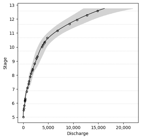
Excercise#
Splines can give unexpectedly poor results. Experiment with the following:
Try changing the random state:
sim_df.sample(n=30, random_state=771)Rerun with
n=200. The fit has improved, but the uncertainty is unreasonably high.Rerun with more degrees of freedon (
df=30) inSplineRating(), and observe how the uncertainty changes.
%load_ext watermark
%watermark -n -u -v -iv -w -p pytensor,xarray
Last updated: Mon Jun 03 2024

Python implementation: CPython
Python version       : 3.11.9
IPython version      : 8.25.0

pytensor: 2.22.1
xarray  : 2024.5.0

pymc       : 5.15.1
arviz      : 0.18.0
numpy      : 1.26.4
ratingcurve: 0.1.dev1+g54c5899

Watermark: 2.4.3