Segmented Power Law

There are several approaches to fitting a stage-discharge rating curve. This notebook demonstrates an simple way to approximate the classic approach, which uses a segmented power law.

# Uncomment below to setup Google Colab. It will take a minute or so.
# %%capture
# !pip install pymc==5.1.2
# %env MKL_THREADING_LAYER=GNU
# !pip install git+https://github.com/thodson-usgs/ratingcurve.git

%load_ext autoreload
%autoreload 2

import pymc as pm
import arviz as az
from ratingcurve.ratings import PowerLawRating

WARNING (pytensor.tensor.blas): Using NumPy C-API based implementation for BLAS functions.

Load Data

Begin by loading the Green Channel dataset

from ratingcurve import data
df = data.load('green channel')
df.head()

	datetime	stage	q	q_sigma
0	2020-05-21 14:13:41 [UTC-07:00]	7.04	12199.342	199.172931
1	2020-04-16 14:55:31 [UTC-07:00]	4.43	4921.953	95.425619
2	2020-03-04 13:54:10 [UTC-07:00]	2.99	2331.665	61.860500
3	2020-03-04 13:16:51 [UTC-07:00]	2.94	2289.220	47.886745
4	2020-01-23 11:04:32 [UTC-07:00]	2.96	2408.210	99.522964

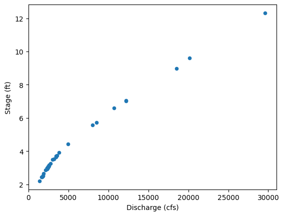
and plotting the observations.

ax = df.plot.scatter(x='q', y='stage', marker='o')
ax.set_xlabel("Discharge (cfs)")
ax.set_ylabel("Stage (ft)")

Text(0, 0.5, 'Stage (ft)')

Setup model

Now, setup the rating model. This make take a minute the first time while the model compiles but will be faster on subsequent runs.

powerrating = PowerLawRating(segments=2,
                             prior={'distribution':'uniform'})

There are of variety of ways to adjust the optimization. Here we’ll use the defaults, which uses ADVI and runs for 200,000 iterations, though the model should coverge well before that.

trace = powerrating.fit(q=df['q'],
                        h=df['stage'], 
                        q_sigma=df['q_sigma'])

/opt/hostedtoolcache/Python/3.11.9/x64/lib/python3.11/site-packages/rich/live.py:231: UserWarning: install 
"ipywidgets" for Jupyter support
  warnings.warn('install "ipywidgets" for Jupyter support')

Convergence achieved at 139500

Interrupted at 139,499 [69%]: Average Loss = 40.4

Sampling: [a, b, hs_, model_q, sigma]

Sampling: [model_q]

/opt/hostedtoolcache/Python/3.11.9/x64/lib/python3.11/site-packages/rich/live.py:231: UserWarning: install 
"ipywidgets" for Jupyter support
  warnings.warn('install "ipywidgets" for Jupyter support')

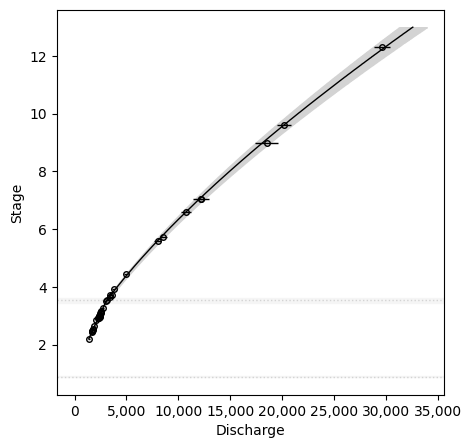
Once fit, we can plot the rating curve.

powerrating.plot()

Sampling: [model_q]

/opt/hostedtoolcache/Python/3.11.9/x64/lib/python3.11/site-packages/rich/live.py:231: UserWarning: install 
"ipywidgets" for Jupyter support
  warnings.warn('install "ipywidgets" for Jupyter support')

or as a table of stage-discharge values.

table = powerrating.table()
table.head()

Sampling: [model_q]

/opt/hostedtoolcache/Python/3.11.9/x64/lib/python3.11/site-packages/rich/live.py:231: UserWarning: install 
"ipywidgets" for Jupyter support
  warnings.warn('install "ipywidgets" for Jupyter support')

	stage	discharge	median	gse
0	2.21	1384.055929	1383.631462	1.017378
1	2.22	1396.196507	1395.951473	1.017410
2	2.23	1408.403309	1408.008281	1.017098
3	2.24	1420.336842	1420.002411	1.017101
4	2.25	1432.380651	1431.898741	1.017345

Exercise

What happens if we choose the wrong number of segments? Increase the number of segments by one and rerun the model. In fact, we can use this to select the correct number of segments, which is demonstrated in the model evaluation notebook.

Simulated Example

This example uses a simulated rating curve, which allows you to test how changing the number of segments affects the rating curve.

First, load the ‘3-segment simulated’ tutorial dataset.

sim_df = data.load('3-segment simulated')

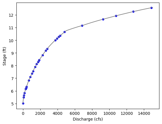
This rating contains observations of every 0.01 inch. increment in stage, which is much more than we’d have for a natural rating. Try sampling to n_sample=15 or n_sample=30 and see how that affects the model fit.

# subsample the simulated rating curve
n_sample = 30
df = sim_df.sample(n_sample, random_state=12345)

ax = sim_df.plot(x='q', y='stage', color='grey', ls='-', legend=False)
df.plot.scatter(x='q', y='stage', marker='o', color='blue', ax=ax)
ax.set_xlabel("Discharge (cfs)");
ax.set_ylabel("Stage (ft)");

Setup a rating model with 3 segments

powerrating = PowerLawRating(segments=3,
                             prior={'distribution':'uniform'},
                             #prior={'distribution':'normal', 'mu':[5, 8, 11], 'sigma':[1, 1, 0.2]}
                            )

now fit the model using ADVI

trace = powerrating.fit(q=df['q'],
                        h=df['stage'],
                        q_sigma=None,
                        method='advi')

/opt/hostedtoolcache/Python/3.11.9/x64/lib/python3.11/site-packages/rich/live.py:231: UserWarning: install 
"ipywidgets" for Jupyter support
  warnings.warn('install "ipywidgets" for Jupyter support')

Finished [100%]: Average Loss = -48.508

Sampling: [a, b, hs_, model_q, sigma]

Sampling: [model_q]

/opt/hostedtoolcache/Python/3.11.9/x64/lib/python3.11/site-packages/rich/live.py:231: UserWarning: install 
"ipywidgets" for Jupyter support
  warnings.warn('install "ipywidgets" for Jupyter support')

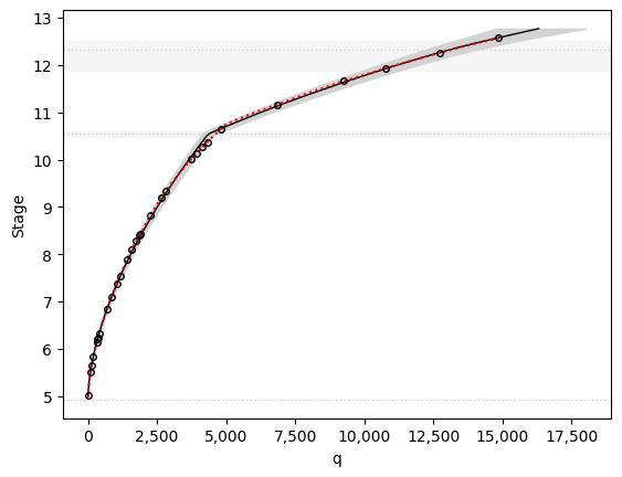
and visualize the results.

import matplotlib.pyplot as plt
fig, ax = plt.subplots()
powerrating.plot(ax=ax)

# plot the original data for comparison
sim_df.plot(x='q', y='stage', color='red', ls=':', legend=False, ax=ax)

Sampling: [model_q]

/opt/hostedtoolcache/Python/3.11.9/x64/lib/python3.11/site-packages/rich/live.py:231: UserWarning: install 
"ipywidgets" for Jupyter support
  warnings.warn('install "ipywidgets" for Jupyter support')

<Axes: xlabel='q', ylabel='Stage'>

powerrating.summary(var_names=["b", "a", "sigma", "hs"])

arviz - WARNING - Shape validation failed: input_shape: (1, 10000), minimum_shape: (chains=2, draws=4)

	mean	sd	hdi_3%	hdi_97%	mcse_mean	mcse_sd	ess_bulk	ess_tail	r_hat
b[0]	0.984	0.002	0.980	0.988	0.000	0.000	9598.0	9163.0	NaN
b[1]	0.353	0.008	0.338	0.368	0.000	0.000	9792.0	9747.0	NaN
b[2]	0.049	0.056	-0.055	0.155	0.001	0.000	10085.0	9675.0	NaN
a	-1.007	0.003	-1.013	-1.002	0.000	0.000	9838.0	9719.0	NaN
sigma	0.015	0.002	0.012	0.019	0.000	0.000	9832.0	9679.0	NaN
hs[0, 0]	4.928	0.001	4.926	4.930	0.000	0.000	10334.0	10066.0	NaN
hs[1, 0]	10.545	0.032	10.486	10.607	0.000	0.000	9758.0	10008.0	NaN
hs[2, 0]	12.317	0.166	12.024	12.532	0.002	0.001	9858.0	9659.0	NaN

Fitting this model can be tricky. The most common issue is a poor initialization of the breakpoints. A fix is under development, but for now, try

1. reinitializing the model PowerLawRating();

2. increasing the number of iterations for the fitting algorithm fit(n=300_000);

3. a prior on the breakpoints, example, try prior={'distribution':'normal', 'mu':[5, 9.5, 10.5], 'sigma':[1, 1, 0.2]}), which implies we know the true breakpoint within +-0.5 ft; or

4. fitting the model with NUTS fit(method='nuts').

%load_ext watermark
%watermark -n -u -v -iv -w -p pytensor,xarray

Last updated: Mon Jun 03 2024

Python implementation: CPython
Python version       : 3.11.9
IPython version      : 8.25.0

pytensor: 2.22.1
xarray  : 2024.5.0

matplotlib : 3.9.0
pymc       : 5.15.1
arviz      : 0.18.0
ratingcurve: 0.1.dev1+g54c5899

Watermark: 2.4.3